Note
Go to the end to download the full example code.
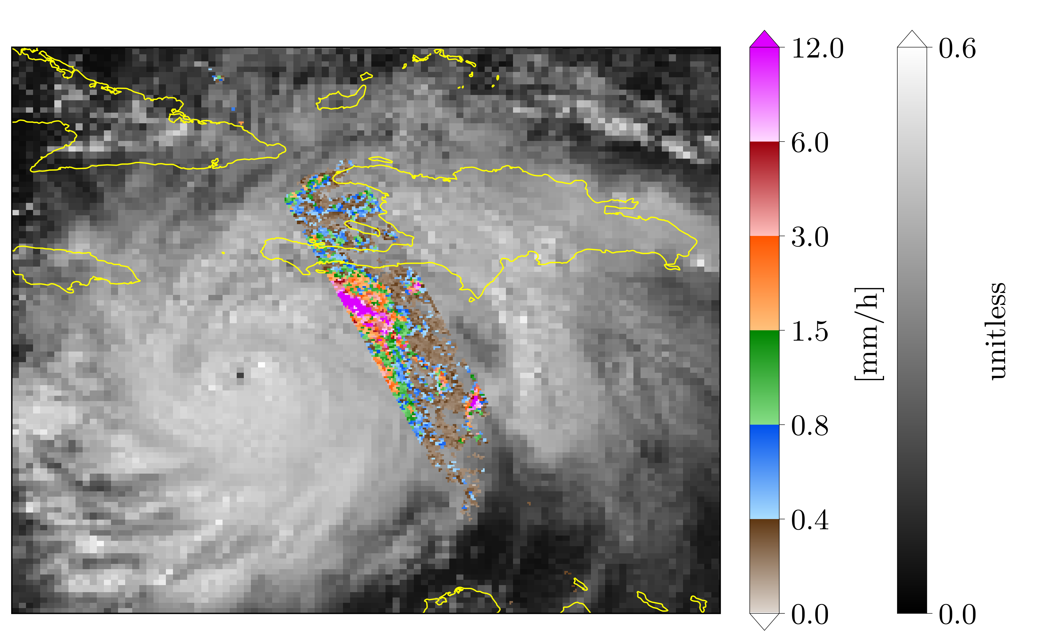
GPM precip rate measurements over Goes Albedo
- Many things are demonstrated in this example:
The superposition of two data types on one figure
Plotting the same data on different domains
The use of the average keyword for displaying high resolution data onto a coarser grid

import numpy as np
import os, inspect
import pickle
import matplotlib as mpl
import matplotlib.pyplot as plt
import cartopy.crs as ccrs
import cartopy.feature as cfeature

# In your scripts use something like :
import domutils.geo_tools as geo_tools
import domutils.legs      as legs

def make_panel(fig, pos, img_res, map_extent, missing,
               dpr_lats, dpr_lons, dpr_pr,
               goes_lats, goes_lons, goes_albedo,
               map_pr, map_goes,
               map_extent_small=None, include_zero=True,
               average_dpr=False):
    ''' Generic function for plotting data on an ax

        Data is displayed with specific projection settings

    '''

    #cartopy crs for lat/lon (ll) and the image (Miller)
    proj_ll  = ccrs.Geodetic()
    proj_mil = ccrs.Miller()

    #global
    #instantiate object to handle geographical projection of data
    #
    #Note the average=True for GPM data, high resolution DPR data
    # will be averaged within coarser images pixel tiles
    proj_inds_dpr = geo_tools.ProjInds(src_lon=dpr_lons, src_lat=dpr_lats,
                                       extent=map_extent, dest_crs=proj_mil,
                                       average=average_dpr, missing=missing,
                                       image_res=img_res)
    proj_inds_goes = geo_tools.ProjInds(src_lon=goes_lons, src_lat=goes_lats,
                                        extent=map_extent, dest_crs=proj_mil,
                                        image_res=img_res, missing=missing)

    ax = fig.add_axes(pos, projection=proj_mil)
    ax.set_extent(proj_inds_goes.rotated_extent, crs=proj_mil)

    #geographical projection of data into axes space
    proj_data_pr   = proj_inds_dpr.project_data(dpr_pr)
    proj_data_goes = proj_inds_goes.project_data(goes_albedo)

    #get RGB values for each data types
    precip_rgb =   map_pr.to_rgb(proj_data_pr)
    albedo_rgb = map_goes.to_rgb(proj_data_goes)

    #blend the two images by hand
    #image will be opaque where reflectivity > 0
    if include_zero:
        alpha = np.where(proj_data_pr >= 0., 1., 0.)  #include zero
    else:
        alpha = np.where(proj_data_pr >  0., 1., 0.)  #exclude zero
    combined_rgb = np.zeros(albedo_rgb.shape,dtype='uint8')
    for zz in np.arange(3):
        combined_rgb[:,:,zz] = (1. - alpha)*albedo_rgb[:,:,zz] + alpha*precip_rgb[:,:,zz]

    #plot image w/ imshow
    x11, x22 = ax.get_xlim()    #get image limits in Cartopy data coordinates
    y11, y22 = ax.get_ylim()
    dum = ax.imshow(combined_rgb, interpolation='nearest',
                    origin='upper', extent=[x11,x22,y11,y22])
    ax.set_aspect('auto')

    #add political boundaries
    ax.add_feature(cfeature.COASTLINE, linewidth=0.8, edgecolor='yellow',zorder=1)

    #plot extent of the small domain that will be displayed in next panel
    if map_extent_small is not None :
        bright_red = np.array([255.,0.,0.])/255.
        w = map_extent_small[0]
        e = map_extent_small[1]
        s = map_extent_small[2]
        n = map_extent_small[3]
        ax.plot([w, e, e, w, w], [s,s,n,n,s],transform=proj_ll, color=bright_red, linewidth=5 )


def main():


    #recover previously prepared data
    currentdir = os.path.dirname(os.path.abspath(inspect.getfile(inspect.currentframe())))
    parentdir  = os.path.dirname(currentdir) #directory where this package lives
    source_file = parentdir + '/test_data/goes_gpm_data.pickle'
    with open(source_file, 'rb') as f:
        data_dict = pickle.load(f)
    dpr_lats    = data_dict['dprLats']
    dpr_lons    = data_dict['dprLons']
    dpr_pr      = data_dict['dprPrecipRate']
    goes_lats   = data_dict['goesLats']
    goes_lons   = data_dict['goesLons']
    goes_albedo = data_dict['goesAlbedo']

    #missing value
    missing = -9999.

    #Figure position stuff
    pic_h = 5.4
    pic_w = 8.8
    pal_sp = .1/pic_w
    pal_w = .25/pic_w
    ratio = .8
    sq_sz = 6.
    rec_w =       sq_sz/pic_w
    rec_h = ratio*sq_sz/pic_h
    sp_w = .1/pic_w
    sp_h = 1.0/pic_h
    x1 = .1/pic_w
    y1 = .2/pic_h

    #number of pixels of the image that will be shown
    hpix = 400.       #number of horizontal pixels E-W
    vpix = ratio*hpix #number of vertical pixels   S-N
    img_res   = (int(hpix),int(vpix))

    mpl.rcParams.update({'font.size': 18})
    mpl.rcParams.update({'font.family':'Latin Modern Roman'})

    #point density for figure
    #Hi def figure
    mpl.rcParams['figure.dpi'] = 400

    #instantiate figure
    fig = plt.figure(figsize=(pic_w,pic_h))

    # Set up colormapping objects

    #For precip rates
    ranges = [0.,.4,.8,1.5,3.,6.,12.]
    map_pr = legs.PalObj(range_arr=ranges,
                         n_col=6,
                         over_high='extend',
                         under_low='white',
                         excep_val=[missing,0.], excep_col=['grey_230','white'])

    #For Goes albedo
    map_goes = legs.PalObj(range_arr=[0., .6],
                           over_high = 'extend',
                           color_arr='b_w', dark_pos='low',
                           excep_val=[-1, missing], excep_col=['grey_130','grey_130'])

    #Plot data on a domain covering North-America
    #
    #
    map_extent = [-141.0, -16., -7.0, 44.0]
    #position
    x0 = x1
    y0 = y1
    pos = [x0,y0,rec_w,rec_h]
    #border of smaller domain to plot on large figure
    map_extent_small = [-78., -68., 12.,22.]
    #
    make_panel(fig, pos, img_res, map_extent, missing,
               dpr_lats, dpr_lons, dpr_pr,
               goes_lats, goes_lons, goes_albedo,
               map_pr, map_goes, map_extent_small,
               average_dpr=True)


    #instantiate 2nd figure
    fig2 = plt.figure(figsize=(pic_w,pic_h))
    # sphinx_gallery_thumbnail_number = 2

    #Closeup on a domain in the viscinity of Haiti
    #
    #
    map_extent = map_extent_small
    #position
    x0 = x1
    y0 = y1
    pos = [x0,y0,rec_w,rec_h]
    #
    make_panel(fig2, pos, img_res, map_extent, missing,
               dpr_lats, dpr_lons, dpr_pr,
               goes_lats, goes_lons, goes_albedo,
               map_pr, map_goes, include_zero=False)


    #plot palettes
    x0 = x0 + rec_w + pal_w
    y0 = y0
    map_pr.plot_palette(pal_pos=[x0,y0,pal_w,rec_h],
                        pal_units='[mm/h]',
                        pal_format='{:2.1f}',
                        equal_legs=True)

    x0 = x0 + 5.*pal_w
    y0 = y0
    map_goes.plot_palette(pal_pos=[x0,y0,pal_w,rec_h],
                          pal_units='unitless',
                          pal_format='{:2.1f}')

    #uncomment to save figure
    #pic_name = 'goes_plus_gpm.svg'
    #plt.savefig(pic_name,dpi=400)


if __name__ == '__main__':
    main()