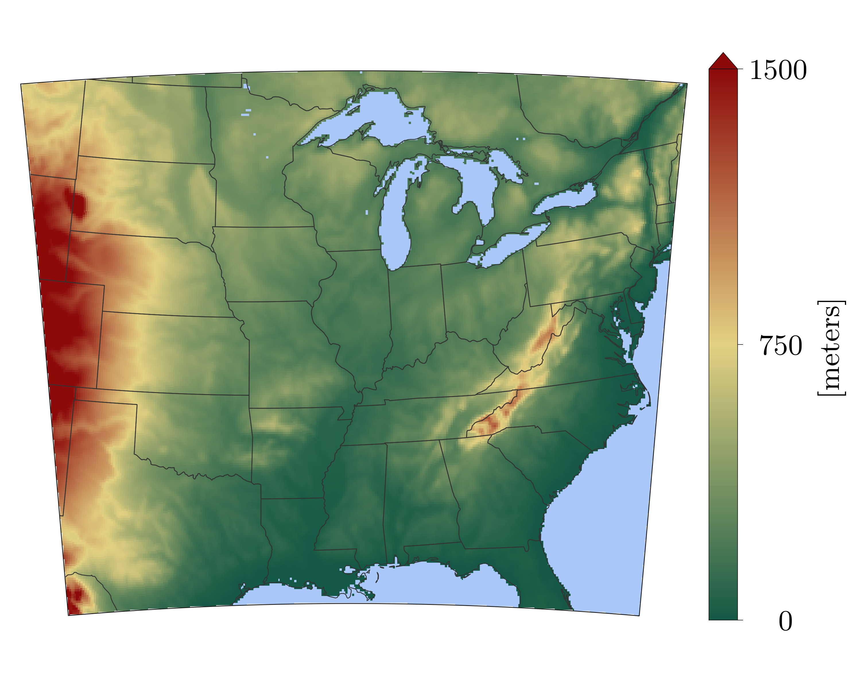
Continuous Qualitative

Continuous and qualitative color mapping for depiction of terrain height in a 10 km version of the Canadian GEM atmospheric model.

import os, inspect
import pickle
import numpy as np
import matplotlib as mpl
import matplotlib.pyplot as plt
import cartopy.crs as ccrs
import cartopy.feature as cfeature

# In your scripts use something like :
import domutils.legs as legs
import domutils.geo_tools as geo_tools



def main():
    #recover previously prepared data
    currentdir = os.path.dirname(os.path.abspath(inspect.getfile(inspect.currentframe())))
    parentdir  = os.path.dirname(currentdir) #directory where this package lives
    source_file = parentdir + '/test_data/pal_demo_data.pickle'
    with open(source_file, 'rb') as f:
        data_dict = pickle.load(f)
    longitudes     = data_dict['longitudes']    #2D longitudes [deg]
    latitudes      = data_dict['latitudes']     #2D latitudes  [deg]
    ground_mask    = data_dict['groundMask']    #2D land fraction [0-1]; 1 = all land
    terrain_height = data_dict['terrainHeight'] #2D terrain height of model [m ASL]

    #flag non-terrain (ocean and lakes) as -3333.
    inds = np.asarray( (ground_mask.ravel() <= .01) ).nonzero()
    if inds[0].size != 0:
        terrain_height.flat[inds] = -3333.

    #missing value
    missing = -9999.

    #pixel density of image to plot
    ratio = 0.8
    hpix = 600.       #number of horizontal pixels E-W
    vpix = ratio*hpix #number of vertical pixels   S-N
    img_res = (int(hpix),int(vpix))

    ##define Albers projection and extend of map
    #Obtained through trial and error for good fit of the mdel grid being plotted
    proj_aea = ccrs.AlbersEqualArea(central_longitude=-94.,
                                    central_latitude=35.,
                                    standard_parallels=(30.,40.))
    map_extent=[-104.8,-75.2,27.8,48.5]

    #point density for figure
    mpl.rcParams['figure.dpi'] = 400
    #larger characters
    mpl.rcParams.update({'font.size': 18})
    mpl.rcParams.update({'font.family':'Latin Modern Roman'})

    #instantiate figure
    fig = plt.figure(figsize=(7.5,6.))

    #instantiate object to handle geographical projection of data
    proj_inds = geo_tools.ProjInds(src_lon=longitudes, src_lat=latitudes,
                                   extent=map_extent,  dest_crs=proj_aea,
                                   image_res=img_res,  missing=missing)

    #axes for this plot
    ax = fig.add_axes([.01,.1,.8,.8], projection=proj_aea)
    ax.set_extent(proj_inds.rotated_extent, crs=proj_aea)

    # Set up colormapping object
    #
    # Two color segments for this palette
    red_green = [[[227,209,130],[ 20, 89, 69]],    # bottom color leg : yellow , dark green
                 [[227,209,130],[140, 10, 10]]]    #    top color leg : yellow , dark red

    map_terrain = legs.PalObj(range_arr=[0., 750, 1500.],
                              color_arr=red_green, dark_pos=['low','high'],
                              excep_val=[-3333.       ,missing],
                              excep_col=[[170,200,250],[120,120,120]],  #blue , grey_120
                              over_high='extend')

    #geographical projection of data into axes space
    proj_data = proj_inds.project_data(terrain_height)

    #plot data & palette
    map_terrain.plot_data(ax=ax,data=proj_data, zorder=0,
                         palette='right', pal_units='[meters]', pal_format='{:4.0f}')   #palette options

    #add political boundaries
    ax.add_feature(cfeature.STATES.with_scale('50m'), linewidth=0.5, edgecolor='0.2',zorder=1)

    #plot border and mask everything outside model domain
    proj_inds.plot_border(ax, mask_outside=True, linewidth=.5)

    #uncomment to save figure
    #plt.savefig('continuous_topo.svg')

if __name__ == '__main__':
    main()